


-
胸径、树高是森林经营和森林调查中的重要因子[1]。在实际调查中,树高的测量耗时费力而且易产生误差[2],而胸径的测量相比树高更加便捷、准确,因此通常只实测部分树木的树高,通过不同树种的树高—胸径模型来预测缺失的树高[3]。关于树高—胸径模型,传统的研究方法通常需要先从较常用的树高曲线模型或其扩展形式中选择若干模型作为候选树高曲线模型,然后分别进行拟合,再根据模型决定系数、参数值等指标,并借助于树高预测-实测对比图、树高预测值-残差图等最终决定适宜的模型[4]。然而候选模型的选择往往依赖于前人研究或由研究者凭经验主观判断,不同研究者选择的候选模型种类、数量都存在较大差异。有的候选模型数量较少,只有几种[4-5],而有的则多达十几种[6]甚至几十种[7],候选模型数量少则精确度不足,数量多则使得工作量加大而效率降低,然而受限于模型本身对数学函数的依赖性以及候选模型数量的有限性,导致其难以最大限度地逼近林分生长的复杂非线性关系。人工神经网络非常适合应用于非线性建模,其在建模过程中不依赖于现存模型并且具有无限逼近任意非线性的能力[8-10]。BP(Back Propagation)人工神经网络是Rumelhart和McCelland领导的科研小组于1986提出的一种按照误差逆向传播算法训练的多层前馈网络,是目前应用最广泛的神经网络模型之一。BP人工神经网络也是林业研究中常用的一种, 马天晓等[11],董云飞等[12]运用BP人工神经网络分别拟合毛白杨(Populus tomentosa Carr.)和杉木(Cunninghamia lanceolata (Lamb.) Hook.)的树高曲线,结果表明BP神经网络具有泛化能力强,精确度高、误差小等优点。
目前应用BP神经网络的研究对象多为人工林[11-13],栎类(Quercus)天然林[14]、兴安落叶松(Larix gmelinii(Rupr.) Kuzen.)天然林[15]等也有应用,但总体来看在天然林中应用较少。本研究以吉林省汪清林业局金沟岭林场的天然云冷杉针阔混交林为对象,分树种(组)通过人工神经网络建立天然云冷杉针阔混交林标准树高模型,并与传统模型进行比较,探讨BP模型在天然针阔混交林中应用的可行性,为森林经营管理中更加高效、准确的建立树高模型提供理论参考。
-
研究区位于吉林省汪清林业局金沟岭林场(130°05'~130°20' E,43°17'~43°25' N)。属长白山系老爷岭山脉雪岭支脉,海拔550~1 100 m,属低山丘陵地带,林场总面积为16 286 hm2。该研究区地处北温带季风区,属大陆性季风型气候,全年平均气温约3.9℃,年积温2 144℃;1月份气温最低,平均在-32℃左右;7月份气温最高,平均在32℃左右。年降水量600~700 mm,且多集中在7月份;植物生长期为120 d左右;山地土壤类型以暗棕壤为主。
-
采用金沟岭林场的12块天然云冷杉针阔混交林样地,每块样地面积为1 hm2。调查样地主要乔木树种有冷杉(Abies nephrolepis(Trautv.) Maxim.)、鱼鳞云杉(Picea jezoensis Carr. var. microsperma(Lindl.)Cheng et L.K.Fu)、红松(Pinus koraiensis Siebold et Zuccarini)、红皮云杉(Picea koraiensis Nakai)、长白落叶松(Larix olgensis Henry)、大青杨(Populus ussuriensis Kom.)、紫椴(Tilia amurensis Rupr.)、色木(Acer mono Maxim.)、黄檗(Phellodendron amurense Rupr.)、榆树(Ulmus pumila Linn.)、白桦(Betula platyphylla Suk.)、水曲柳(Fraxinus mandschurica Rupr.)和枫桦(Betula costata Trautv.)等。实测树高1.3 m以上树木的胸径和树高,共得到观测数据12 953对。为便于建模,将树种进行分组,其中:落叶松1 303对,云杉(包括鱼鳞云杉和红皮云杉,下同)1 073对,冷杉3 111对,红松965对,慢阔(色木、水曲柳、黄檗、紫椴和枫桦)4 335对,中阔(白桦、大青杨、榆树和杂木)2 141对数据。选择其中8块样地的数据用于建模,剩下的4块样地数据用于模型检验,取样地中树高最大的100棵树的平均树高作为林分优势高,数据概况见表 1。
表 1 建模和验证数据概况(模拟样地8块,检验样地4块)
Table 1. Summary of statistics of 8 modeling plots and 4 test plots
树种(组)
Tree species
(groups)建模样地Modeling plots 检验样地Test plots 两种样地数据曼惠特
尼U检验
Mann-Whitney U test数据类型
Data type平均值
Mean标准差
SD最大值
Max最小值
Min平均值
Mean标准差
SD最大值
Max最小值
Min落叶松
Larix olgensisD/cm 21.1 6.3 43.3 2.3 18.3 4.3 34.8 5.4 极显著very significant H/m 21.7 4.5 34.2 2.4 20.3 3.7 28.7 7.6 极显著very significant Ht/m 25.1 1.2 27.0 23.7 24.9 0.4 25.2 24.2 极显著very significant 云杉
Picea spp.D/cm 16.1 10.9 55.5 1.0 14.0 9.5 56.0 1.0 极显著very significant H/m 13.3 7.8 33.0 1.7 12.1 7.2 28.8 1.5 极显著very significant Ht/m 25.1 1.2 27.0 23.7 24.9 0.4 25.2 24.2 极显著very significant 冷杉
Abies nephrolepisD/cm 10.0 8.9 53.0 1.0 9.4 8.5 40.3 1.0 极显著very significant H/m 9.0 7.3 31.0 1.6 8.9 7.3 28.2 1.5 极显著very significant Ht/m 25.1 1.2 27.0 23.7 24.9 0.4 25.2 24.2 极显著very significant 红松
Pinus koraiensisD/cm 16.9 12.0 54.0 1.0 17.8 11.1 72.0 1.0 不显著not significant H/m 12.8 7.1 28.0 1.5 13.6 6.2 25.9 1.7 不显著not significant Ht/m 25.1 1.2 27.0 23.7 24.9 0.4 25.2 24.2 极显著very significant 慢阔
deciduous tree group 1D/cm 13.0 8.4 54.3 1.0 13.9 8.5 53.2 1.2 极显著very significant H/m 19.2 21.9 32.2 1.0 14.3 6.8 31.1 2.1 极显著very significant Ht/m 25.1 1.2 27.0 23.7 24.9 0.4 25.2 24.2 极显著very significant 中阔
deciduous tree group 2D/cm 12.2 8.1 54.8 1.2 15.1 9.6 46.2 2.0 极显著very significant H/m 12.4 6.3 32.7 2.1 14.7 7.6 34.4 3.4 极显著very significant Ht/m 25.1 1.2 27.0 23.7 24.9 0.4 25.2 24.2 极显著very significant 注:D为胸径,H为单木树高,Ht为林分优势高, 慢阔包括色木、水曲柳、黄檗、紫椴和枫桦,中阔包括白桦、大青杨、榆树和杂木。D is diameter at breast height, H is individual tree height, Ht is dominant height, deciduous tree group 1 includes mono maple (Acer mono), ash (Fraxinus mandschurica), amur corktree (Phellodendron amurense), amur linden (Tilia amurensis), ribbed birch (Betula costata), deciduous tree group 2 includes white birch (Betula platyphylla), poplar (Populus ussuriensis), elm (Ulmus pumila) and weedtrees. -
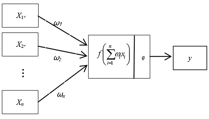
BP网络的拓扑结构包括:输入层、隐层和输出层(图 1),输入层将刺激信号传送到隐藏层,隐藏层由神经元之间联系的强弱(权重)和传递规则(激活函数)将刺激信号传送到输出层,输出层整合隐藏层处理后的刺激产生最终结果。如果存在正确结果,则比较正确结果和产生结果得出误差,然后逆推对神经网中的链接权重进行反馈修正,进而完成神经网络的学习过程。神经元的结构模型见图 2,(x1、x2、…、xn)为神经元的输入量,y为神经元的输出(也是下一层神经元的输入),(ω1、ω2、…、ωn)为权值,θ为阀值,f为激活函数,$ y = f\left( {\sum\limits_{i = 1}^n {{\omega _i}} {x_i}} \right)$。根据Kolmogorov定理,单隐层BP网络就能无限逼近任何连续的非线性曲线[16]。
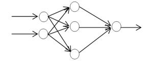
图 1 单隐层BP神经网络结构图
Figure 1. BP neural network structure of single hidden layer
图 2 神经元结构图
Figure 2. BP neure structure
-
基于Matlab(2014b)及软件自带的nntool工具箱建立单隐层BP神经网络模型以估测树高,其中,网络的输入层为胸径和林分优势高,输出层为树高,根据经验,BP神经网络隐层节点数可用Nh=$ \sqrt {{N_{in}} + {N_{out}}} $+h计算[17],式中:Nh为隐层节点数;Nin、Nout分别为输入层和输出层节点数;h取1~10之间的整数)来确定取值范围。本研究采用试凑法在此范围内逐个取值,根据拟合精度确定隐层节点。节点数确定后就可以得到模型的适宜结构,简化表现为Nin:Nh:Nout。
数据在参与建模前需要进行归一化处理,以加快训练网络的收敛速度,公式为:Y=(X-Min)/(Max-Min)(式中X、Y分别为转换前和转换后的值,Max、Min分别为样本的最大值、最小值)。
建模时,设置学习速率为0.01,目标精度为0.001,最大迭代次数为1 000,以logsig函数(Y=1/(1+e-x),X,Y分别为自变量和因变量)作为隐层神经元传递函数,以purelin函数(Y=aX+b,X,Y分别为自变量和因变量) 作为输出层传递函数,以Levenberg—Marquardt法作为训练算法。
-
根据前人的研究,从传统树高曲线研究中选择了两个应用较广的代表性模型:传统模型1:H=1.3+aDbe-c/Ht式中H为树高,D为胸径,Ht为林分优势高,a、b、c为参数[5];传统模型2:H=1.3+(a+bHt)/(c+D) 式中H为树高,D为胸径,Ht为林分优势高,a、b、c为参数[18]。
-
使用决定系数(R2)、平均绝对误差(MAE)和均方根误差(RMSE)来评价模型精度。决定系数越大、平均绝对误差、均方根误差越小,模型拟合精度越高。
-
构建以胸径和林分优势高作为输入变量,树高为输出变量,隐层节点数为Nh的BP神经网络。由经验公式计算得出Nh在2.732~11.732之间,为增加模型的容错性将隐层节点数范围稍稍扩大即调整为2~11的整数值,分树种(组)根据试凑法依次取节点数为2到11,每个节点训练20次并计算对应的平均R2和平均RMSE(见表 2)。由结果可知,R2随节点数的增大而增大,而RMSE随节点数增大而减小,也即:隐层节点数越大,模型精度越高。
表 2 各树种(组)不同隐层节点数的20次拟合统计量均值
Table 2. Average statistics of fitting 6 tree species (groups) with different hidden layers for 20 times
树种(组)
Tree species
(group)落叶松
Larix olgensis云杉
Picea spp.冷杉
Abies nephrolepis红松
Pinus koraiensis慢阔
Deciduous tree
group 1中阔
Deciduous tree
group 2节点数
Nodes决定
系数
R2均方根
误差
RMSE决定
系数
R2均方根
误差
RMSE决定
系数
R2均方根
误差
RMSE决定
系数
R2均方根
误差
RMSE决定
系数
R2均方根
误差
RMSE决定
系数
R2均方根
误差
RMSE2 0.608 5 2.823 9 0.902 4 2.437 8 0.922 6 2.057 9 0.922 0 2.143 8 0.790 5 2.861 6 0.810 4 2.751 2 3 0.627 6 2.773 8 0.903 1 2.422 1 0.923 3 2.022 5 0.923 4 1.993 1 0.790 8 2.859 1 0.811 7 2.743 1 4 0.636 4 2.746 8 0.903 9 2.408 3 0.924 8 2.010 6 0.924 4 1.981 9 0.792 2 2.854 9 0.812 3 2.725 8 5 0.636 9 2.739 9 0.904 4 2.398 7 0.925 7 1.990 6 0.925 7 1.957 7 0.793 2 2.853 4 0.813 3 2.722 4 6 0.637 1 2.722 1 0.905 2 2.376 0 0.927 5 1.962 8 0.926 7 1.941 3 0.794 4 2.849 8 0.814 6 2.723 3 7 0.638 7 2.729 4 0.906 8 2.364 5 0.928 6 1.961 3 0.927 3 1.933 1 0.795 1 2.848 3 0.815 2 2.717 8 8 0.639 7 2.711 9 0.907 7 2.354 3 0.930 5 1.925 6 0.928 2 1.931 8 0.786 2 2.846 6 0.816 0 2.702 7 9 0.640 5 2.707 0 0.908 4 2.334 4 0.931 7 1.906 8 0.929 7 1.930 8 0.797 9 2.845 2 0.816 9 2.702 4 10 0.645 0 2.700 4 0.909 6 2.323 9 0.932 9 1.903 5 0.931 0 1.925 1 0.798 2 2.843 4 0.818 1 2.701 0 11 0.646 4 2.695 5 0.910 3 2.312 2 0.933 0 1.856 8 0.932 4 1.920 9 0.799 8 2.827 0 0.819 4 2.688 1 由于隐层节点数不能为无限大,为进一步确定隐藏节点数,将神经网络的输出变量(树高)与其对应的输入变量(胸径)建立散点图,当散点图出现失真现象时说明此时模型的隐层节点数已不可取。图 3为落叶松、云杉、冷杉、红松、慢阔、中阔在隐层节点数分别为6、6、9、5、8、5时的散点图,图中反映胸径-树高关系的点所组成的曲线出现了不同程度的分化以及变形,因此判定此时的图像出现了失真现象。综合考虑模型的简化性和实用性,故选择图像失真时隐层节点数的前一个作为最佳隐层节点数,即落叶松、云杉、冷杉、红松、慢阔、中阔的隐层节点数分别为5、5、8、4、7、4。

图 3 失真时胸径-树高散点图
Figure 3. Scatter diagram of D-H when distortion happened
-
节点数确定后,经过不断重复的训练,选择适宜的结构Nin:Nh:Nout作为最终模型,得到相应神经网络模型的传递函数表达式如下:
(1) 落叶松:适宜模型结构(即输入层节点数:隐藏层节点数:输出层节点数)为2:5:1
$ \begin{array}{l} H = {\rm{ purelin }}\left( {0.4639 - 0.1248{h_1} + 0.0928{h_2} - } \right.\\ \left. {0.0115{h_3} - 1.3626{h_4} - 1.3940{h_5}} \right){\rm{。}}\\ {h_1} = \log {\mathop{\rm sig}\nolimits} ( - 6.4395 + 5.6027D + 2.8373Ht);\\ {h_2} = \log {\mathop{\rm sig}\nolimits} ( - 0.3741 - 3.7381D + 12.0065Ht);\\ {h_3} = \log {\mathop{\rm sig}\nolimits} ( - 0.1719 - 3.7007D - 6.5111Ht);\\ {h_4} = \log {\mathop{\rm sig}\nolimits} ( - 6.4343 - 3.8270D + 0.9123Ht);\\ {h_5} = \log {\mathop{\rm sig}\nolimits} ( - 1.8855 - 3.1314D + 0.0887Ht); \end{array} $
(2) 云杉:适宜模型结构为2:5:1
$ \begin{array}{l} H = {\rm{ purelin }}\left( { - 1.1715 + 0.0430{h_1} + 0.1128{h_2} + 0.} \right.\\ \left. {0626{h_3} + 1.6016{h_4} - 0.1197{h_5}} \right){\rm{。}}\\ {h_1} = {\mathop{\rm logsig}\nolimits} ( - 2.1693 - 27.6447D + 27.9251Ht);\\ {h_2} = \log {\mathop{\rm sig}\nolimits} ( - 11.9033 - 8.2726D - 2.6794Ht);\\ {h_3} = {\mathop{\rm logsig}\nolimits} ( - 15.2527 + 46.7691D + 0.8751Ht);\\ {h_4} = {\mathop{\rm logsig}\nolimits} (2.9820 + 4.6421D - 0.0380Ht){\rm{;}}\\ {h_5} = \log {\mathop{\rm sig}\nolimits} (20.8359 + 0.7357D + 13.4391Ht); \end{array} $
(3) 冷杉:适宜模型结构为2:8:1
$ \begin{array}{l} H = {\mathop{\rm purelin}\nolimits} \left( {0.1452 + 0.1727{h_1} + 0.2398{h_2} + 0.2770{h_3}} \right.\\ - 0.5670{h_4} - 1.1561{h_5} + 0.0204{h_6} + 0.1363{h_7} + \\ \left. {0.3266{h_8}} \right){\rm{。}}\\ {h_1} = {\mathop{\rm logsig}\nolimits} ( - 9.8685 + 0.7250D + 6.5268Ht);\\ {h_2} = {\mathop{\rm logsig}\nolimits} ( - 6.4640 + 7.1473D + 0.3082Ht);\\ {h_3} = {\mathop{\rm logsig}\nolimits} (4.9614 - 9.2452D + 3.9107Ht);\\ {h_4} = {\mathop{\rm logsig}\nolimits} ( - 1.0353 - 3.9014D - 1.2716Ht);\\ {h_5} = {\mathop{\rm logsig}\nolimits} ( - 3.5565 - 5.2224D + 0.6099Ht);\\ {h_6} = {\mathop{\rm logsig}\nolimits} (9.0301 + 16.9134D + 0.9483Ht);\\ {h_7} = \log {\mathop{\rm sig}\nolimits} (1.6082 - 1.4568D + 9.4052Ht);\\ {h_8} = \log {\mathop{\rm sig}\nolimits} ( - 5.9476 + 9.0265D - 8.9319Ht); \end{array} $
(4) 红松:适宜模型结构为2:4:1
$ \begin{array}{l} H = {\mathop{\rm purelin}\nolimits} \left( {0.7225 + 3.2092{h_1} + 0.2280{h_2} - 0.1886{h_3}} \right.\\ \left. { - 2.0123{h_4}} \right){\rm{。}}\\ {h_1} = \log {\mathop{\rm sig}\nolimits} ( - 11.9252 + 4.7827D + 1.6905Ht);\\ {h_2} = \log {\mathop{\rm sig}\nolimits} ( - 22.4803 + 9.2799D + 13.6115Ht);\\ {h_3} = {\mathop{\rm logsig}\nolimits} (0.6089 + 0.1705D - 3.1494Ht);\\ {h_4} = {\mathop{\rm logsig}\nolimits} ( - 2.4162 - 3.7589D + 0.1508Ht); \end{array} $
(5) 慢阔(色木、水曲柳、黄檗、紫椴和枫桦):适宜模型结构为2:7:1
$ \begin{array}{l} H = {\rm{ purelin }}\left( { - 1.2278 + 1.2961{h_1} - 1.3039{h_2} + } \right.\\ 0.3929{h_3} - 1.0262{h_4} + 0.6911{h_5} + 1.1451{h_6} + 0.\\ \left. {8502{h_7}} \right){\rm{。}}\\ {h_1} = \log {\mathop{\rm sig}\nolimits} ( - 7.2323 + 6.0538D + 2.9312Ht);\\ {h_2} = \log {\mathop{\rm sig}\nolimits} ( - 1.104 - 0.7832D - 1.9373Ht);\\ {h_3} = \log {\mathop{\rm sig}\nolimits} (1.1871 - 0.0592D - 8.5434Ht);\\ {h_4} = \log {\mathop{\rm sig}\nolimits} (2.0342 - 2.0373D + 8.1388Ht);\\ {h_5} = \log {\mathop{\rm sig}\nolimits} (1.4719 - 3.2549D + 11.7175Ht);\\ {h_6} = \log {\mathop{\rm sig}\nolimits} (4.0818 + 5.5186D - 0.2693Ht);\\ {h_7} = \log {\mathop{\rm sig}\nolimits} (7.8083 + 5.9249D - 0.8637Ht); \end{array} $
(6) 中阔(白桦、大青杨、杂木和榆树)适宜模型结构为2:4:1
$ \begin{array}{l} H = {\rm{ purelin }}\left( {12.994 - 13.4257{h_1} - 1.0191{h_2} + 0.} \right.\\ \left. {0744{h_3} + 0.9451{h_4}} \right){\rm{。}}\\ {h_1} = {\mathop{\rm logsig}\nolimits} (14.9234 - 9.8915D - 5.9081Ht);\\ {h_2} = \log {\mathop{\rm sig}\nolimits} ( - 10.0509 - 10.3678D + 0.1648Ht);\\ {h_3} = \log {\mathop{\rm sig}\nolimits} ( - 13.1296 - 5.0691D + 14.9891Ht);\\ {h_4} = \log {\mathop{\rm sig}\nolimits} (5.7266 + 8.1656D + 0.0337Ht); \end{array} $
以上式中,H为树高值;hi为隐层神经元的传递输出;i = 1,2…;purelin为线性函数;logsig为对数S型函数;D和Ht分别为胸径和林分优势高。
-
根据所选用的胸径和林分优势高,在传统树高曲线研究中选择了两个模型(传统模型1和传统模型2),运用相同的8块建模样地数据预估各参数值,将建模样地数据代入到3个模型中,并比较其建模表现(表 3)。由表 3可知,BP神经网络的R2均大于传统模型,MAE和RMSE均小于传统模型,可见BP模型的拟合效果优于传统模型。
表 3 BP模型与传统模型建模精度比较
Table 3. Comparison of performances between BP model and traditional models with 8 modeling plots
树种(组)
Tree species(group)模型
Models平均绝对误差
MAE决定系数
R2均方根误差
RMSE落叶松 模型1 model 1 2.003 2 0.595 0 2.872 8 Larix olgensis 模型2 model 2 2.031 7 0.594 9 2.873 2 BP 1.974 3 0.635 5 2.721 6 云杉 模型1 model 1 1.515 3 0.895 4 2.515 6 Picea spp. 模型2 model 2 1.754 1 0.876 5 2.732 8 BP 1.501 8 0.910 6 2.323 9 冷杉 模型1 model 1 1.602 8 0.909 5 2.193 3 Abies nephrolepis 模型2 model 2 1.405 6 0.903 7 2.262 9 BP 1.244 1 0.930 5 1.925 6 红松 模型1 model 1 1.674 7 0.910 4 2.135 3 Pinus koraiensis 模型2 model 2 1.796 6 0.895 1 2.310 4 BP 1.532 9 0.922 4 1.981 9 慢阔 模型1 model 1 2.491 7 0.779 6 2.930 1 Deciduous tree 模型2 model 2 2.674 3 0.770 8 2.850 6 group 1 BP 2.443 1 0.794 1 2.844 8 中阔 模型1 model 1 2.316 6 0.781 3 2.946 8 Deciduous tree 模型2 model 2 2.172 6 0.805 7 2.777 8 group 2 BP 2.076 2 0.817 9 2.684 1 注:模型1 H=1.3+aDbe-c/Ht式中H为树高,D为胸径,Ht为林分优势高,a、b、c为参数[5]。
Model 1 H=1.3+aDbe-c/Ht, H is tree height, D is diameter at breast height, Ht is dominant height, a, b and c are parameters.
模型2 H=1.3+(a+bHt)/(c+D)式中H为树高,D为胸径,Ht为林分优势高,a、b、c为参数[18]。
Model 2 H=1.3+(a+bHt)/(c+D), H is tree height, D is diameter at breast height, Ht is dominant height, a, b and c are parameters.运用相同的4块检验样地数据代入到3个模型中,计算出相应的平均绝对误差(MAE)和均方根误差(RMSE)并比较其表现(表 4)。由表 4可知,BP神经网络的MAE和RMSE分别在1.251 8~2.454 6、2.006 0~3.1273之间,且均小于传统模型,可见BP模型的精度比传统的方程要高。
表 4 BP模型与传统模型误差比较
Table 4. Comparison of error analysis between BP model and traditional models with 4 test plots
树种(组)
Tree species(group)模型
Models平均绝对误差
MAE均方根误差
RMSE落叶松 模型1 model 1 2.017 0 2.630 2 Larix olgensis 模型2 model 2 2.051 2 2.633 6 BP 1.986 7 2.587 3 云杉 模型1 model 1 1.523 1 2.146 0 Picea spp. 模型2 model 2 1.776 1 2.290 6 BP 1.512 3 2.122 0 冷杉 模型1 model 1 1.614 1 2.140 8 Abies nephrolepis 模型2 model 2 1.418 7 2.101 9 BP 1.251 8 2.006 0 红松 模型1 model 1 1.683 5 2.207 5 Pinus koraiensis 模型2 model 2 1.804 9 2.317 1 BP 1.543 6 2.172 9 慢阔 模型1 model 1 2.503 8 3.178 4 Deciduous tree 模型2 model 2 2.683 1 3.350 1 group 1 BP 2.454 6 3.127 3 中阔 模型1 model 1 2.321 4 3.062 8 Deciduous tree 模型2 model 2 2.181 1 2.906 6 group 2 BP 2.081 1 2.828 9 图 4为使用随机选取的6块样地(其中2块样地的林分优势树高比较接近)数据代入BP模型中的预测结果。可以看出,在林分优势高一定的情况下,胸径越大,树高越大;在胸径一定的条件下,树高随林分优势高增大而增大。模型表现符合树木生长的客观规律。
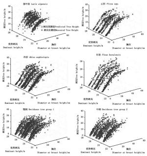
图 4 随机样地数据预测树高与实际树高比较
Figure 4. Comparison between predicted tree height and measured tree height using data from random 6 plots
-
本文中BP模型的R2均大于传统模型,MAE、RMSE均小于传统模型,这与陈建珍等[19]研究所得结果类似,说明BP模型拟合精度高于传统模型,误差小于传统模型,体现了BP模型在建模方面的优越性。分树种(组)来看,云杉、冷杉、红松的R2要高于慢阔、中阔,针叶树种(除落叶松)明显大于阔叶树种,这与卢军等[7]的研究相一致,这是因为云杉、冷杉、红松为地带性顶级树种,将在地带性顶级群落中占据为优势树种[20],其生长过程受到影响较少,规律性更强。
本文建立模型的预测变量仅包含胸径和林分优势高。林分优势高可以在一定程度上反映林分的立地条件,但树木树高的生长受到多种因子的共同影响,除林分优势高外,还应该考虑将林分因子(密度、竞争等),气候因子(温度、降水、光照等)等变量加入到模型中,这样可以提高模型的预测精度。在实际应用BP模型预测树高时,最理想的方式是在MATLAB中导入研究对象的胸径、林分优势高等数据,借助nntool工具箱,自行建立一个针对当地特定研究对象的BP神经网络模型,这种建模过程全程在nntool工具箱中进行可视化操作,全程不涉及编程,方便实用;若研究区条件、树种等与本文类似的,还可以直接使用本文中所建立的BP模型(或者参数数据)以节省一些中间步骤。然而从原理上看BP神经网络是通过已知数据建立一个空间映射关系,但其内部结构并不清楚,可以理解为一个黑箱,在应用中缺少相应的生物学解释,这成为限制BP模型应用的重要因素。
-
本研究以汪清林业局金沟岭林场12块天然云冷杉针阔混交林样地为对象,基于matlab平台分树种(组)构建了以胸径和林分优势高为输入量,树高为输出量的输入一输出BP神经网络标准树高模型,并得到各树种(组)的最佳模型,落叶松的R2=0.635 5,适宜模型结构(即输入层节点数:隐藏层节点数:输出层节点数)为2:5:1;云杉的R2=0.910 6,适宜模型结构为2:5:1;冷杉的R2=0.930 5,适宜模型结构为2:8:1;红松的R2=0.922 4,适宜模型结构为2:4:1;慢阔的R2=0.794 1,适宜模型结构为2:7:1;中阔的R2=0.817 9,适宜模型结构为2:4:1。与传统树高模型建模方式相比,BP模型不依赖已知函数,不需要在前期筛选模型形式,减小了建模工作量并避免了由研究者主观判断所产生的误差,而且BP模型对树木生长的非线性关系可以无限逼近,因此也提高了模型精度。从模型的拟合及预测效果上看,BP模型各树种R2相比传统模型有所提高,MAE、RMSE等误差指标有所降低,因此BP神经网络总体表现要稍优于传统方法,BP模型可以有效地预测树高。
基于BP神经网络的天然云冷杉针阔混交林标准树高-胸径模型
Generalized Height-diameter Model for Natural Mixed Spruce-fir Coniferous and Broadleaf Forests based on BP Neural Network
-
摘要:
目的 以吉林省汪清林业局金沟岭林场12块天然云冷杉针阔混交林样地为对象,基于12 953对实测树高-胸径数据,结合林分优势高分树种(组)建立基于BP神经网络的标准树高模型。 方法 在确定隐层节点数后经过反复训练得到各树种(组)的适宜模型结构,使用相同的建模数据(8块样地)求解两个传统的树高方程,再利用未参与建模的4块样地分别验证模型。 结果 表明:落叶松、云杉的适宜模型结构(输入层节点数:隐藏层节点数:输出层节点数)为2:5:1;红松、中阔(白桦、大青杨、榆树和杂木)的适宜模型结构为2:4:1;冷杉的适宜模型结构为2:8:1;慢阔(色木、水曲柳、黄檗、紫椴和枫桦)的适宜模型结构为2:7:1。 结论 与传统方法相比,BP模型不依赖现存函数,不需要筛选模型形式,而且BP模型各树种R2高于传统模型,平均绝对误差、均方根误差均小于传统模型,其拟合精度和预测效果均优于传统方程,可以有效地预测树高。 -
关键词:
- BP神经网络
- / 天然云冷杉针阔混交林
- / 标准树高-胸径模型
Abstract:Objective Twelve plots of natural mixed spruce-fir coniferous and broadleaf forests located in Jin'gouling Forest Farm of Jilin Province were investigated to establish height prediction models for main tree species based on 12 953 data of tree height, diameter and dominant height by using BP neural network. Method After determining the hidden nodes, an optimum model structure was developed by training BP models of Larix olgensis, Picea spp., Abies nephrolepis, Pinus koraiensis and two deciduous groups repeatedly. Then, they were compared with two traditional height-diameter equations in which the parameters were solved with the same input datasets from 8 plots to establish BP models, and the validation datasets from the other 4 plots were used to test the models. Result The results show that the optimal network structure of L. olgensis and Picea spp. (nodes in input layers: nodes in hidden layers: nodes in output layers) are both 2:5:1, the optimal network structure of Pinus koraiensis, one deciduous group (Betula platyphylla, Populus ussuriensis, Ulmus pumila and other tree species) are both 2:4:1, the optimal network structure of A. nephrolepis is 2:8:1, and the optimal network structure of the other deciduous group (Acer mono, Fraxinus mandschurica, Phellodendron amurense, Tilia amurensis, and Betula costata) is 2:7:1. Conclusion Compared with traditional methods, the BP models need not rely on existing functions or choose model forms. The R2 of BP models are higher than that of the traditional models, and both the mean absolute error and root mean square error of BP models are less than that of the traditional models. The fitting accuracy and prediction effect of BP neural network models are better than those of traditional equations, and thus can predict tree height effectively. -
图 4 随机样地数据预测树高与实际树高比较
Figure 4. Comparison between predicted tree height and measured tree height using data from random 6 plots
表 1 建模和验证数据概况(模拟样地8块,检验样地4块)
Table 1. Summary of statistics of 8 modeling plots and 4 test plots
树种(组)
Tree species
(groups)建模样地Modeling plots 检验样地Test plots 两种样地数据曼惠特
尼U检验
Mann-Whitney U test数据类型
Data type平均值
Mean标准差
SD最大值
Max最小值
Min平均值
Mean标准差
SD最大值
Max最小值
Min落叶松
Larix olgensisD/cm 21.1 6.3 43.3 2.3 18.3 4.3 34.8 5.4 极显著very significant H/m 21.7 4.5 34.2 2.4 20.3 3.7 28.7 7.6 极显著very significant Ht/m 25.1 1.2 27.0 23.7 24.9 0.4 25.2 24.2 极显著very significant 云杉
Picea spp.D/cm 16.1 10.9 55.5 1.0 14.0 9.5 56.0 1.0 极显著very significant H/m 13.3 7.8 33.0 1.7 12.1 7.2 28.8 1.5 极显著very significant Ht/m 25.1 1.2 27.0 23.7 24.9 0.4 25.2 24.2 极显著very significant 冷杉
Abies nephrolepisD/cm 10.0 8.9 53.0 1.0 9.4 8.5 40.3 1.0 极显著very significant H/m 9.0 7.3 31.0 1.6 8.9 7.3 28.2 1.5 极显著very significant Ht/m 25.1 1.2 27.0 23.7 24.9 0.4 25.2 24.2 极显著very significant 红松
Pinus koraiensisD/cm 16.9 12.0 54.0 1.0 17.8 11.1 72.0 1.0 不显著not significant H/m 12.8 7.1 28.0 1.5 13.6 6.2 25.9 1.7 不显著not significant Ht/m 25.1 1.2 27.0 23.7 24.9 0.4 25.2 24.2 极显著very significant 慢阔
deciduous tree group 1D/cm 13.0 8.4 54.3 1.0 13.9 8.5 53.2 1.2 极显著very significant H/m 19.2 21.9 32.2 1.0 14.3 6.8 31.1 2.1 极显著very significant Ht/m 25.1 1.2 27.0 23.7 24.9 0.4 25.2 24.2 极显著very significant 中阔
deciduous tree group 2D/cm 12.2 8.1 54.8 1.2 15.1 9.6 46.2 2.0 极显著very significant H/m 12.4 6.3 32.7 2.1 14.7 7.6 34.4 3.4 极显著very significant Ht/m 25.1 1.2 27.0 23.7 24.9 0.4 25.2 24.2 极显著very significant 注:D为胸径,H为单木树高,Ht为林分优势高, 慢阔包括色木、水曲柳、黄檗、紫椴和枫桦,中阔包括白桦、大青杨、榆树和杂木。D is diameter at breast height, H is individual tree height, Ht is dominant height, deciduous tree group 1 includes mono maple (Acer mono), ash (Fraxinus mandschurica), amur corktree (Phellodendron amurense), amur linden (Tilia amurensis), ribbed birch (Betula costata), deciduous tree group 2 includes white birch (Betula platyphylla), poplar (Populus ussuriensis), elm (Ulmus pumila) and weedtrees.  下载: 导出CSV
表 2 各树种(组)不同隐层节点数的20次拟合统计量均值
Table 2. Average statistics of fitting 6 tree species (groups) with different hidden layers for 20 times
树种(组)
Tree species
(group)落叶松
Larix olgensis云杉
Picea spp.冷杉
Abies nephrolepis红松
Pinus koraiensis慢阔
Deciduous tree
group 1中阔
Deciduous tree
group 2节点数
Nodes决定
系数
R2均方根
误差
RMSE决定
系数
R2均方根
误差
RMSE决定
系数
R2均方根
误差
RMSE决定
系数
R2均方根
误差
RMSE决定
系数
R2均方根
误差
RMSE决定
系数
R2均方根
误差
RMSE2 0.608 5 2.823 9 0.902 4 2.437 8 0.922 6 2.057 9 0.922 0 2.143 8 0.790 5 2.861 6 0.810 4 2.751 2 3 0.627 6 2.773 8 0.903 1 2.422 1 0.923 3 2.022 5 0.923 4 1.993 1 0.790 8 2.859 1 0.811 7 2.743 1 4 0.636 4 2.746 8 0.903 9 2.408 3 0.924 8 2.010 6 0.924 4 1.981 9 0.792 2 2.854 9 0.812 3 2.725 8 5 0.636 9 2.739 9 0.904 4 2.398 7 0.925 7 1.990 6 0.925 7 1.957 7 0.793 2 2.853 4 0.813 3 2.722 4 6 0.637 1 2.722 1 0.905 2 2.376 0 0.927 5 1.962 8 0.926 7 1.941 3 0.794 4 2.849 8 0.814 6 2.723 3 7 0.638 7 2.729 4 0.906 8 2.364 5 0.928 6 1.961 3 0.927 3 1.933 1 0.795 1 2.848 3 0.815 2 2.717 8 8 0.639 7 2.711 9 0.907 7 2.354 3 0.930 5 1.925 6 0.928 2 1.931 8 0.786 2 2.846 6 0.816 0 2.702 7 9 0.640 5 2.707 0 0.908 4 2.334 4 0.931 7 1.906 8 0.929 7 1.930 8 0.797 9 2.845 2 0.816 9 2.702 4 10 0.645 0 2.700 4 0.909 6 2.323 9 0.932 9 1.903 5 0.931 0 1.925 1 0.798 2 2.843 4 0.818 1 2.701 0 11 0.646 4 2.695 5 0.910 3 2.312 2 0.933 0 1.856 8 0.932 4 1.920 9 0.799 8 2.827 0 0.819 4 2.688 1
下载: 导出CSV
表 3 BP模型与传统模型建模精度比较
Table 3. Comparison of performances between BP model and traditional models with 8 modeling plots
树种(组)
Tree species(group)模型
Models平均绝对误差
MAE决定系数
R2均方根误差
RMSE落叶松 模型1 model 1 2.003 2 0.595 0 2.872 8 Larix olgensis 模型2 model 2 2.031 7 0.594 9 2.873 2 BP 1.974 3 0.635 5 2.721 6 云杉 模型1 model 1 1.515 3 0.895 4 2.515 6 Picea spp. 模型2 model 2 1.754 1 0.876 5 2.732 8 BP 1.501 8 0.910 6 2.323 9 冷杉 模型1 model 1 1.602 8 0.909 5 2.193 3 Abies nephrolepis 模型2 model 2 1.405 6 0.903 7 2.262 9 BP 1.244 1 0.930 5 1.925 6 红松 模型1 model 1 1.674 7 0.910 4 2.135 3 Pinus koraiensis 模型2 model 2 1.796 6 0.895 1 2.310 4 BP 1.532 9 0.922 4 1.981 9 慢阔 模型1 model 1 2.491 7 0.779 6 2.930 1 Deciduous tree 模型2 model 2 2.674 3 0.770 8 2.850 6 group 1 BP 2.443 1 0.794 1 2.844 8 中阔 模型1 model 1 2.316 6 0.781 3 2.946 8 Deciduous tree 模型2 model 2 2.172 6 0.805 7 2.777 8 group 2 BP 2.076 2 0.817 9 2.684 1 注:模型1 H=1.3+aDbe-c/Ht式中H为树高,D为胸径,Ht为林分优势高,a、b、c为参数[5]。
Model 1 H=1.3+aDbe-c/Ht, H is tree height, D is diameter at breast height, Ht is dominant height, a, b and c are parameters.
模型2 H=1.3+(a+bHt)/(c+D)式中H为树高,D为胸径,Ht为林分优势高,a、b、c为参数[18]。
Model 2 H=1.3+(a+bHt)/(c+D), H is tree height, D is diameter at breast height, Ht is dominant height, a, b and c are parameters.
下载: 导出CSV
表 4 BP模型与传统模型误差比较
Table 4. Comparison of error analysis between BP model and traditional models with 4 test plots
树种(组)
Tree species(group)模型
Models平均绝对误差
MAE均方根误差
RMSE落叶松 模型1 model 1 2.017 0 2.630 2 Larix olgensis 模型2 model 2 2.051 2 2.633 6 BP 1.986 7 2.587 3 云杉 模型1 model 1 1.523 1 2.146 0 Picea spp. 模型2 model 2 1.776 1 2.290 6 BP 1.512 3 2.122 0 冷杉 模型1 model 1 1.614 1 2.140 8 Abies nephrolepis 模型2 model 2 1.418 7 2.101 9 BP 1.251 8 2.006 0 红松 模型1 model 1 1.683 5 2.207 5 Pinus koraiensis 模型2 model 2 1.804 9 2.317 1 BP 1.543 6 2.172 9 慢阔 模型1 model 1 2.503 8 3.178 4 Deciduous tree 模型2 model 2 2.683 1 3.350 1 group 1 BP 2.454 6 3.127 3 中阔 模型1 model 1 2.321 4 3.062 8 Deciduous tree 模型2 model 2 2.181 1 2.906 6 group 2 BP 2.081 1 2.828 9
下载: 导出CSV
-
[1] Lei X, Peng C, Wang H, et al. Individual height-diameter models for young black spruce(Picea mariana) and jack pine(Pinus banksiana) plantations in New Brunswick, Canada[J]. The Forestry Chronicle, 2009, 85(1): 43-56. doi: 10.5558/tfc85043-1 [2] Colbert K C, Larsen D R, Lootens J R. Height-diameter equations for thirteen Midwestern bottomland hardwood species[J]. Northern Journal of Applied Forestry, 2002, 19(4): 171-176. doi: 10.1093/njaf/19.4.171 [3] Sharma M, Parton J. Height-diameter equations for boreal tree species in Ontario using a mixed-effects modeling approach[J]. Forest Ecology and Management, 2007, 249(3): 187-198. doi: 10.1016/j.foreco.2007.05.006 [4] 李海奎, 法蕾. 基于分级的全国主要树种树高-胸径曲线模型[J]. 林业科学, 2011, 47(10): 83-90. [5] 王明亮, 唐守正. 标准树高曲线的研制[J]. 林业科学研究, 1997, 10(3): 259-264. doi: 10.3321/j.issn:1001-1498.1997.03.006 [6] 马武, 雷相东, 徐光, 等. 蒙古栎天然林单木生长模型的研究: Ⅱ. 树高-胸径模型[J]. 西北农林科技大学学报: 自然科学版, 2015, 43(3): 83-90. [7] 卢军, 张会儒, 雷相东, 等. 长白山云冷杉针阔混交林幼树树高-胸径模型[J]. 北京林业大学学报, 2015, 37(11): 10-25. [8] 傅荟璇. Matlab神经网络应用设计[M]. 北京: 机械工业出版社, 2010: 94-95. [9] 浦瑞良, 宫鹏, Yang R. 应用神经网络和多元回归技术预测森林产量[J]. 应用生态学报, 1999, 10(2): 129-134. [10] 林辉, 彭长辉. 人工神经网络在森林资源管理中的应用[J]. 世界林业研究, 2002, 15(3): 22-31. [11] 马天晓, 赵晓峰, 黄家荣, 等. 基于人工神经网络的树高曲线模型研究[J]. 河南林业科技, 2006, 26(1): 4-5. [12] 董云飞, 孙玉军, 王轶夫, 等. 基于BP神经网络的杉木标准树高曲线[J]. 东北林业大学学报, 2014, 42(7): 154-156, 165. [13] 车少辉, 张建国, 段爱国, 等. 杉木人工林胸径生长神经网络建模研究[J]. 西北农林科技大学学报: 自然科学版, 2012, 40(3): 84-92. [14] 黄旭光. 基于人工神经网络的栎树天然林生长动态模拟系统研究[D]. 郑州: 河南农业大学, 2014. [15] 金星姬, 贾炜玮, 李凤日. 基于BP人工神经网络的兴安落叶松天然林全林分生长模型的研究[J]. 植物研究, 2008, 28(3): 370-374. [16] Nakamura M, Mines R, Kreinovich V. Guaranteed intervals for Kolmogorov's theorem (and their possible relation to neural networks)[J]. Interval Computations, 1993, 3: 183-199. [17] 张立明. 人工神经网络的模型及其应用[M]. 上海: 复旦大学出版社, 1993: 43-46. [18] 胥辉, 全宏波, 王斌, 等. 思茅松标准树高曲线的研究[J]. 西南林学院学报, 2000, 20(2): 74-77. [19] 陈建珍. BP神经网络在林分平均胸径生长预估中的应用[J]. 林业调查规划, 2009, 34(3): 8-11. [20] 龚直文. 长白山退化云冷杉林演替动态及恢复研究[D]. 北京: 北京林业大学, 2009. -

 点击查看大图

计量
- 文章访问数: 3821
- HTML全文浏览量: 920
- PDF下载量: 802
- 被引次数: 0
