


-
森林结构体现了林木个体 (结构要素)及其属性 (种类、大小、位置) 的连接方式[1],森林结构的异质性可使森林群落中树种多样性增加,促使森林具有更高的稳定性及完整性[2-3],维持森林结构多样性同时被认为是保护生物多样性的最佳途径[4-7]。森林生态系统具有典型的三维特征,组成林分整体的林木个体及其在空间中的排列方式决定了森林系统的属性特征以及功能[8-9],分析群落中种群个体在空间中的分布状态,以及林木个体与其周围相邻木的组织方式、种内种间相互关系以及所处生境的异质性是近年来森林生物物理结构研究的热点之一。
由于环境的异质性、林木间的竞争、种子传播机制等多种因素导致林木位置分布的多样性,采用点格局分析方法可描述林木位置随尺度的变化特征[10-14],如运用Ripley K函数,O-ring统计,双相关函数等分析林木的空间分布格局和不同树种的空间相关性,但这些方法大多数仅对林木的位置信息进行了分析,没有包含林木的其它属性,很难与具体的生态学过程相联系。将树种、胸径、树高、冠幅和存活状态等属性标记在林木的位置上,采用标记点格局分析方法即可描述林木属性随尺度变化的特征[15-18],如运用标记相关函数和标记变异函数分析树种、胸径、树高或径向生长在相应尺度上林木属性的相似性和空间自相关性[19-20],可以提供更多的森林空间结构信息。此外,还可以通过构建标记来分析林木间的关系。构建标记通常有差异标记、比例标记、产量标记等,郝珉辉等[20]以林木生长量为标记,运用标记相关函数研究了阔叶红松林林木生长的空间相关性,认为树种生长特征的空间关联格局具有明显的生境依赖性。Pommerening等[17, 21-22]基于标记相关函数的构造原理,提出了标记混交度和标记大小分化二阶特征函数,有效避免了NNSS方法中相邻木选择数量的问题,可解释林分中树种的排列状态和大小分化随尺度变化的情况,同时,对一些生态学过程和假说具有一定的分析和解释能力[23-24],Wang等[25]运用标记混交度二阶结构特征发现阔叶红松林中大树具有较大的混交度,在一定程度上解释了负密度效应假说。本研究运用单变量双相关函数分析4块面积为1 hm2的阔叶红松林每木定位样地的林木分布格局特征,然后运用标记双相关函数、标记变异函数、标记混交度二阶特征和标记大小分化阶特征函数联合分析树种和林木大小分化特征,从不同的角度分析不同类型阔叶红松林的空间结构特征,探讨阔叶红松林结构形成的生态过程,以期为进一步保护和培育阔叶红松林,维持生物多样性提供参考。
-
研究区位于吉林省吉林市蛟河林业实验区管理局东大坡经营区内,43°51′~44°05′ N, 127°35′~127°51′ E,气候属温带大陆性季风山地气候,分布最广的地带性土壤是肥力较高的暗棕壤,植被类型属于温带针阔混交林区域——温带针阔混交林地带—长白山地红松、杉松针阔混交林区,主要针叶树种有:红松 (Pinus koraiensis Sieb. et Zucc.)、鱼鳞云杉(Picea jezoensis var microsperma (Lindl))、杉松 (Abies holophylla Maxim)、和臭冷杉(Abies nephrolepis (Trautv) Maxim.);主要阔叶树种有:核桃楸(Juglans mandshurica Maxim)、水曲柳 (Fraxinus mandshurica Rupr.)、色木槭 (Acer mono Maxim.)、千金榆 (Carpinus cordata Bl.)、白扭槭 (Acer mandshurica Maxim.)、紫椴 (Tilia amurensis Rupr.)、暴马丁香(Syringa reticulate var. mandshurica (Maxim. Hara))、蒙古栎 (Quercus mongolica Fisch.)、青楷槭 (A. tegmentosum Maxim)等;常见下木有刺五加(Acanthopanax senticossus (Rupr. et Maxim) Harms)、楔叶绣线菊窄叶变种(Spiraea canescens var. sublanceolata Rehd.)和胡枝子(Lespedeza bicolor Turcz)、等;主要草本植物有蕨类(Adiantum spp.)、小叶芹(Aegopodium alpestre Ledeb.)、苔草(Carex spp.)、山茄子(Brachybotrys paridiformis Maxim.)、蚊子草(Filipendula spp.)等。
-
2007年5月到2008年10月期间,根据蛟河林业实验区管理局东大坡经营区林班划分情况,在现地踏查的基础上,在试验区建立了4块面积为100 m × 100 m的固定样地,运用全站仪对样地内胸径大于5 cm的林木进行定位,调查林木的胸径、树种、树高等,同时记载林分的郁闭度、坡度、坡向等因子;在样地内四角及中心设置了5个10 m × 10 m的小样方,调查样方内的幼苗、幼树情况。在内业分析时,将样地按树种断面积的组成情况依次编号为A、B、C、D(表1),4块样地代表了4种类型的阔叶红松林,即样地A为核桃楸和沙松为主的针阔混交林,样地B为以核桃楸、水曲柳和红松为主的针阔混交林,样地C为水曲柳和红松为主的针阔混交林,样地D为以核桃楸、色木槭和沙松为主的针阔混交林。
表 1 4块样地林分基本特征
Table 1. The basic characteristics of fourdifferent samples
样地
Plot坡度
Slope/(°)海拔
Altitude/m郁闭度
Canopy closure密度
Density/
(trees·hm−2)平均树高
Mean height/m平均胸径
Mean DBH/cm断面积
Basal area/
(m2·hm−2)树种数量
Number of spcices树种组成
Tree compositionsA 9 620 0.90 797 13.7 22.5 31.671 19 3核桃楸2沙松1色木槭1红松4其它 B 8 600 0.85 936 13.8 19.8 28.740 19 3核桃楸3水曲柳1红松3其它 C 9 600 0.9 816 13.6 21.5 29.564 22 3水曲柳2红松1核桃楸4其它 D 9 620 0.85 748 13.1 21.8 27.952 21 2核桃楸1色木槭1榆树1沙松5其它 -
单变量双相关函数(UPCF)g(r)、标记相关函数(MCF)
$ {\widehat{K}}_{mm}\left(r\right) $ 和标记变异函数(MVF)$ {\widehat{\gamma }}_{m}\left(r\right) $ 等3个函数在以往的研究中已经应用很多[19-20],其中,g(r)用来分析林木的空间点格局;$ {\widehat{K}}_{mm}\left(r\right) $ 和$ {\widehat{\gamma }}_{m}\left(r\right) $ 用来分析群落标记特征(如林木大小等)的空间相关性特征,二者采用不同的测试函数和归一化方法,$ {\widehat{K}}_{mm}\left(r\right) $ 以标记属性特征的乘积作为测试函数,即$ {f}_{2}({m}_{i},{m}_{j})={m}_{i}{m}_{j} $ ,相应的期望值为林分算术平均胸径的平方(μ2);当$ {\widehat{K}}_{mm}\left(r\right)<1 $ ,表明在距离为$ r $ 的范围内的林木大小属性特征趋向于小于平均值;当$ {\widehat{K}}_{mm}\left(r\right)>1 $ 时,距离为$ r $ 的范围内的林木标记特征趋向于大于平均值;而$ {\widehat{\gamma }}_{m}\left(r\right) $ 则表达标记特征随着尺度的变异程度,其测试函数为$ {f}_{1}\left({m}_{i},{m}_{j}\right)= $ $ 0.5{({m}_{i}-{m}_{j})}^{2} $ ;当$ {\widehat{\gamma }}_{m}\left(r\right)<1 $ 时,表明在距离为$ r $ 的范围内相似大小林木有聚集的特征;当$ {\widehat{\gamma }}_{m}\left(r\right)>1 $ 时,表明在距离为$ r $ 的范围内相似大小林木间排斥,而不同大小的林木聚集。 -
Pommerening等[21]基于标记相关函数的构造原理,以Gadow提出的简单混交度及大小分化度分别作为测试函数[26],其中,标记大小分化度二阶特征测试函数表达式为:
$ t\left({m}_{1},{m}_{2}\right)=1-\dfrac{{\rm{min}}\left\{{m}_{1},{m}_{2}\right\}}{{\rm{max}}\left\{{m}_{1},{m}_{2}\right\}} $
(1) 式中,
$ {m}_{1} $ 和$ {m}_{2} $ 是标记在两个不同林木位置上的林木大小定量属性值,由于林木胸径测量容易且能够稳定代表林木的大小属性特征,因此本研究中以林木胸径值计算。林分中每株树可作为参照树,将其胸径值($ {m}_{1} $ )与其距离为r的相邻木($ {m}_{2} $ )进行比较,可构建标记大小分化二阶特征检验函数:$\begin{split} &\hat \tau \left( r \right) = \frac{1}{{ET}}\mathop \sum \limits_{{x_1},{x_{2 \in W}}}^ \ne \\ &\frac{{(1-{\rm{min}}\left\{ {m\left( {{x_1}} \right),m\left( {{x_2}} \right)} \right\}/{\rm{max}}\left\{ {m\left( {{x_1}} \right),m\left( {{x_2}} \right)} \right\}){k_h}\left( {\parallel {x_1}-{x_2}\parallel-r} \right)}}{{2\pi rA\left( {{W_{{x_1}}}\mathop \cap {W_{{x_2}}}} \right)}} \end{split}$
(2) 式中,
$ {x}_{1} $ 和$ {x}_{2} $ 是在所观测的窗口中两个任意的点。k为Epanechnikovkenel核函数,$ A({W}_{{x}_{1}}\cap {W}_{{x}_{2}}) $ 为$ {W}_{{x}_{1}} $ 与$ {W}_{{x}_{2}} $ 相交面积,用于矩形样地的边缘矫正。当标记大小分化度$ \widehat{\tau }\left(r\right)=1 $ 时,表示群落中林木大小随机分布;当$ \widehat{\tau }\left(r\right)>1 $ 时,表示群落中不同大小林木个体聚集或相似大小林木排斥;当$ \widehat{\tau }\left(r\right)<1 $ 时,表示群落中相似大小林木个体聚集或不同大小林木个体排斥。ET为期望大小分化度,其计算过程首先将样地中林木胸径由小到大进行排序:$ {m}_{1}\le {m}_{2}\le \dots \le {m}_{N} $ 。然后定义一个累加变量Di,其表达式为:$ {D_i}{\rm{ = }}\left\{ {\begin{aligned} &{0\;\;\;\;\;\;\;\;\;\;\;\;\;\;\;\;\;\;\;\;\;\;\;\;\;{\rm{for}}\;\;i = 1,}\\ &{{m_1} + \cdots + {m_i}\;{\rm{for}}\;i = 2, \cdots N.} \end{aligned}} \right. $
(3) 根据样地林木数量N及上式中的Di可得到林分期望大小分化值为:
$ {{E}}T=1-\frac{2}{N(N-1)}{\sum }_{i=1}^{N}\frac{{D}_{i}}{{m}_{i}} $
(4) 同样,将混交度的指示函数作为测试函数可构建标记混交度二阶特征。其中测试函数表达式为:
$ {M}_{i}={\bf{1}}({m}_{1}\ne {m}_{2}) $
(5) 式中,
$ {m}_{1} $ 和$ {m}_{2} $ 是标记在两个不同位置上的林木树种属性值。式(5)为指示函数,当$ {m}_{1} $ 和$ {m}_{2} $ 为不同树种时,$ {M}_{i} $ 值为1,否则其值为0。标记混交度二阶特征检验函数表达式为:
$ \hat \nu \left( r \right) = \frac{1}{{EM}}\sum\limits_{{x_1},{x_{2 \in W}}}^ \ne{\frac{{1\left( {m\left( {{x_1}} \right)\nem\left( {{x_2}} \right)} \right){k_h}(\parallel {x_1}-{x_2}\parallel-r)}}{{2\pi rA({W_{{x_1}}} \cap {W_{{x_2}}})}}} $
(6) 式中,
${x}_{1}{\text{、}}{x}_{2}$ 是在所观测的窗口中两个任意的点。$ A $ $ ({W}_{{x}_{1}}\cap {W}_{{x}_{2}}) $ 为边缘矫正权重,$ {k}_{h} $ 为Epanechnikovkenel核函数。EM为期望混交度,因此当标记混交度的$ \widehat{\nu }\left(r\right) $ 的值等于1时,表达了群落中的树种间随机分布;当$ \widehat{\nu }\left(r\right)>1 $ 时,表达了不同树种聚集或同种排斥;当$ \widehat{\nu }\left(r\right)<1 $ 时,为相同树种聚集或不同树种间负相关。其中,林分的期望混交度计算为:$ {E}M={\sum }_{i=1}^{s}\frac{{N}_{i}\left(N-{N}_{i}\right)}{N\left(N-1\right)} $
(7) 其中s为树种数,N为样地林木株数,Ni为第i个树种的林木个数。
-
本研究在进行二阶特征乘积密度估计时采用Epanechnikovkenel函数(
$ {k}_{h} $ ),其中$ {k}_{h} $ 的带宽既不能设置的太窄,也不能太宽,太窄时包含在圆环中的点太少,会造成随机波动,而太宽时包含太多的点,则会忽视了所关注的尺度距离r处的特征。本研究根据样地的密度将带宽统一设置为2 m。在进行林木分布格局分析时,采用完全空间随机过程(CSR)均质泊松过程作为零模型;在对标记胸径二阶特征分析时,采用随机标记零模型,即保持林木的位置坐标不变,将标记属性随机分配到林木的位置上[17]。在进行标记混交度二阶特征分析时,采用了随机叠加或种群独立性检验[17, 21, 27];对于多树种混交的林分而言,设置一组树种的位置固定不变,移动另一组树种,两组树种林木个数约为总数的一半。对于标记大小分化二阶特征分析时仍随机标记零模型。运用蒙特卡洛完全随机分布模型重复1 000次,模拟产生95%的置信区间,并绘制上限和下限分别为2.5%和97.5%的包迹线,对标记函数结果偏离随机状态的进行显著性检验。在数据计算和分析时,均使用R统计软件进行。标记双相关函数、标记变异函数、标记混交度和标记大小分化度相关代码文件可在Pommerening森林生物实验室(Pommerening's Forest Biometrics Lab)获得。为避免边缘效应对结果的影响,采用NN1方法进行边缘校正[28]。
-
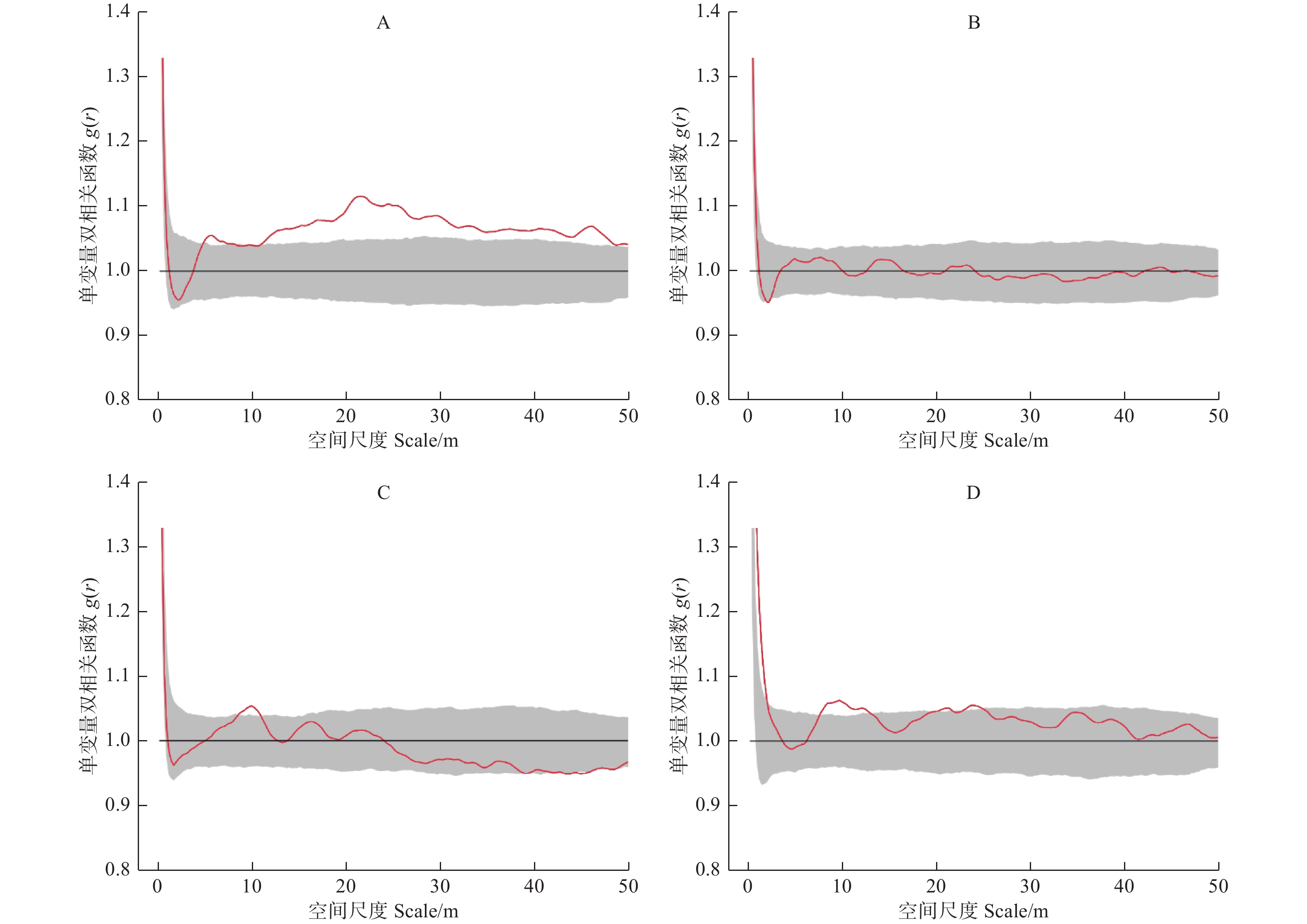
单变量双相关函数g(r)结果表明(图1),4块样地中的林木分布格局存在一定的差异。样地A中的林木在r = 5~8 m的尺度上和r大于10 m的尺度上,林木呈现显著聚集的格局特征;样地B中林木的分布格局整体上为随机分布;样地C和样地D分别在r = 8~11 m和r = 7~12 m的尺度上呈现显著聚集分布的趋势,而在其他尺度上林木的分布格局为随机分布。
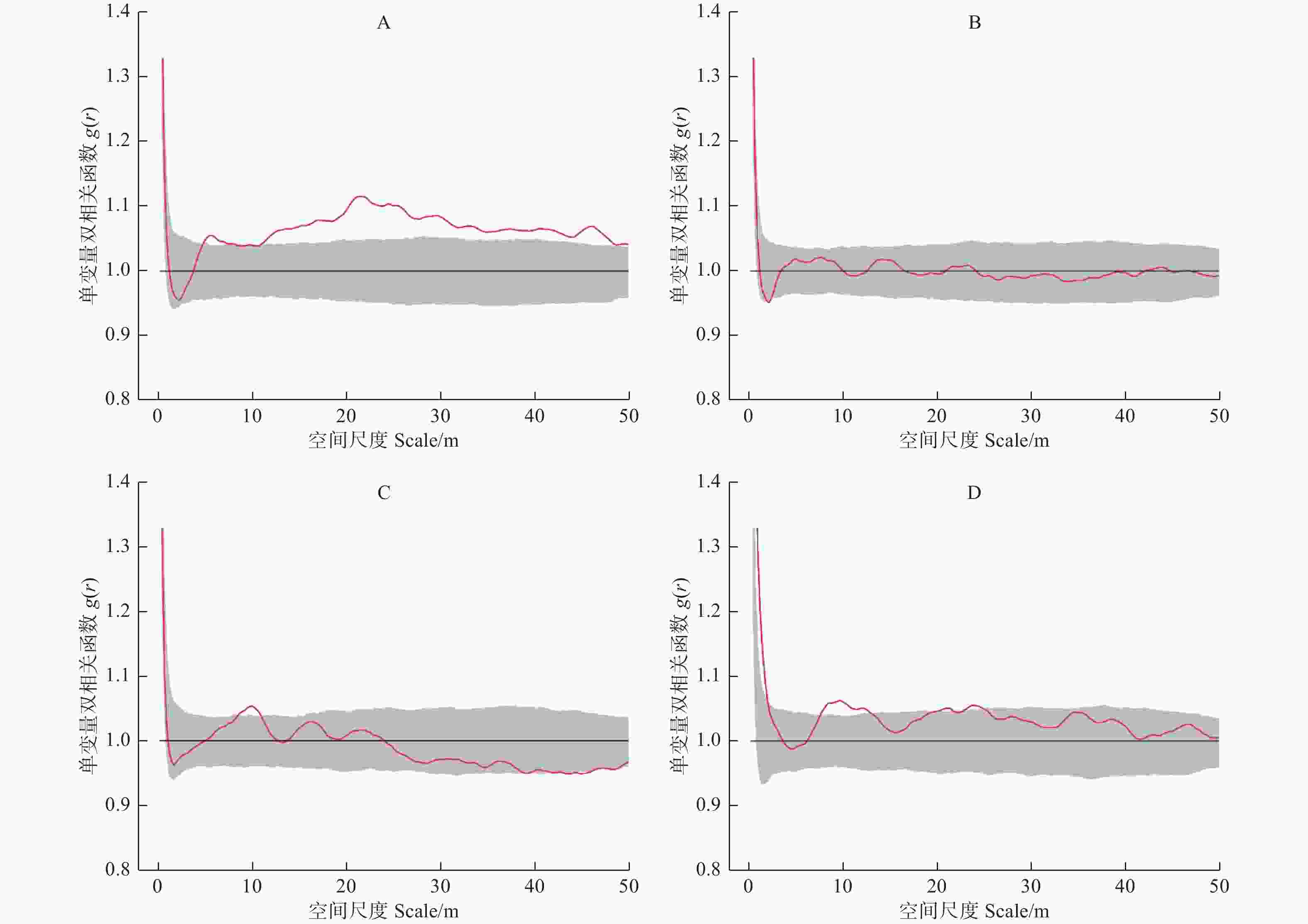
图 1 样地林木分布格局随尺度变化
Figure 1. Spatial distribution pattern of trees with scale
-
以胸径为标记的相关函数表明(图2左),样地A中的林木在r = 0~50 m的观察尺度上,标记胸径相关函数
$ {\widehat{K}}_{mm}\left(r\right) $ 的观测值都小于1,同时在r = 0~8 m和r = 13~33 m的尺度上小于随机标记零模型,表明成对相邻木具有小树特征;样地B、C和D标记相关函数结果非常类似,即$ {\widehat{K}}_{mm}\left(r\right) $ 的观测值在小尺度上小于1,随着研究尺度的增加,$ {\widehat{K}}_{mm}\left(r\right) $ 的观测值在1附近波动,说明这几个样地中的林木在小尺度上表现出相邻木多为小树,其中,样地B、C和D分别在r = 0~8 m,r = 0~7 m和r = 0~6 m的尺度上较为显著,而在其它尺度上林木的胸径大小随机分布。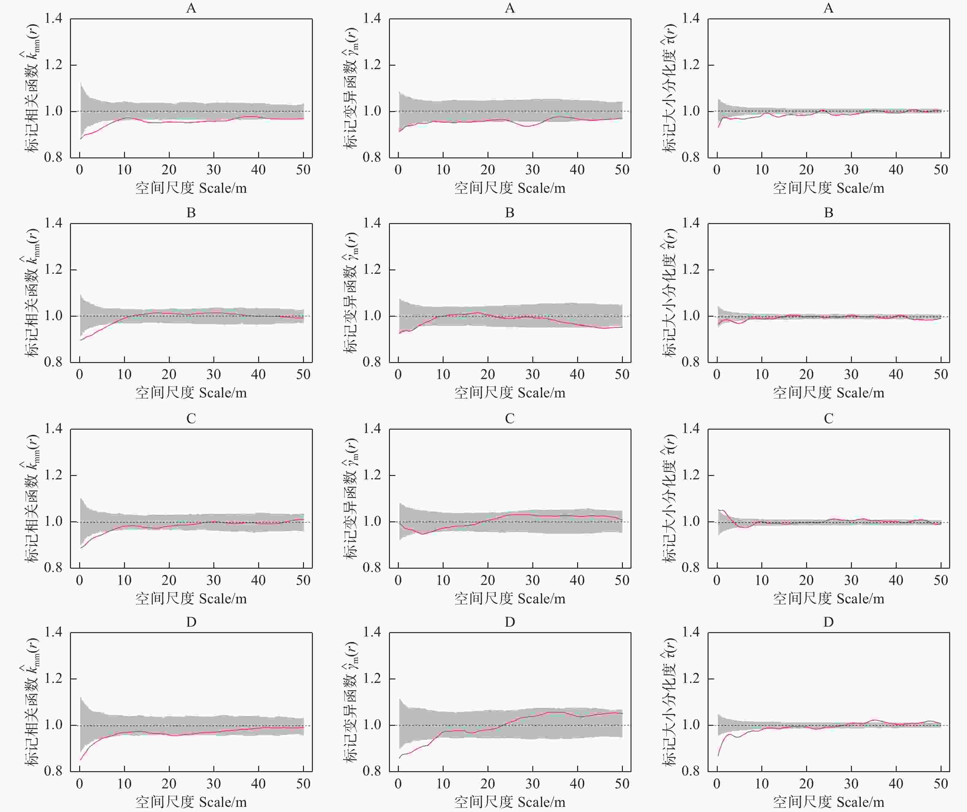
图 2 不同类型阔叶红松林胸径标记二阶特征
Figure 2. Second-order characteristics of DBH markers in different types of broad-leaved Korean pine forests
-
标记胸径变异函数结果表明(图2中),样地A中的林木在r = 0~50 m的观察尺度上,
$ \widehat{\gamma }\left(r\right) $ 的观测值均都小于1,说明样地A中的林木在对应尺度上林木具有相似胸径聚集的趋势,随机标记零模型检验表明,在r = 25~33 m的尺度上这种趋势较为显著。样B和样地C中的林木在r = 0~50 m的观察尺度上,标记胸径变异函数$ \widehat{\gamma }\left(r\right) $ 的观测值始终变化在1的附近波动,完全落入了包迹线内,表明这2块样地内林木胸径大小相关性不明显;样地D内的林木在标记胸径变异函数$ \widehat{\gamma }\left(r\right) $ 的观测值在小尺度上小于1,随着尺度的增加趋向于在1的附近波动,样地D内的林木在r = 0~9 m的尺度上呈现显著的空间正自相关,即相似胸径大小的林木聚集分布,而在其它尺度上林木胸径大小呈现空间上不相关的特征。 -
不同类型阔叶红松林标记大小分化二阶特征函数表明(图2右),4块样地中的林木大小分化特征并未完全落在零模型内,说明4块样地内不同大小林木的分布并非是完全随机分布的格局。其中,样地A内林木的标记大小分化二阶特征函数
$ \widehat{\tau }\left(r\right) $ 观测值在不同尺度下小于1,说明林木胸径的大小分化度显著小于期望大小分化度,相似大小的林木聚集在一起;样地B和D样地内林木的标记大小分化度二阶特征表现出类似的趋势,即这2块样地仅在小尺度上表现出相似大小林木显著聚集的特征,对应的尺度分别为r = 4~6 m和r = 0~12 m;同时样地D内林木的标记大小分化度在r = 0~12 m的尺度上观察值与期望值相差较大。与其他样地不同,样地C内林木的标记大小分化度二阶特征函数$ \widehat{\tau }\left(r\right) $ 的值在r = 0~5 m的尺度上大于1,表明林木胸径的大小分化度大于期望大小分化度,意味着不同大小的林木聚集在一起,即小树与大树吸引,小树与小树排斥。 -
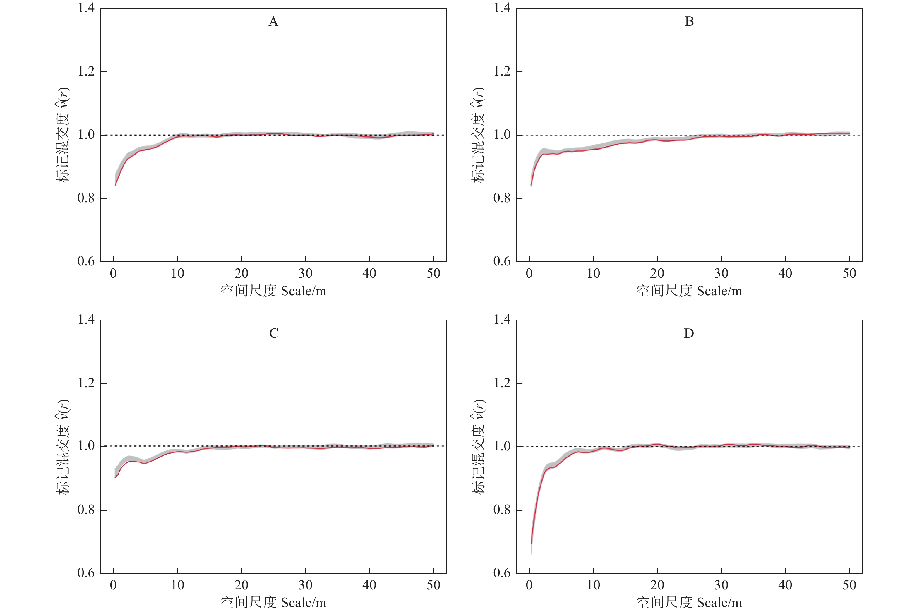
根据随机叠加(或种群独立性)零模型(图3)结果表明,4块样地内的树种整体分布属于完全随机分布,标记混交度二阶函数
$ \widehat{\nu }\left(r\right) $ 的观测值在一定的尺度范围内均小于1,并且随着研究尺度的增加,其值逐渐接近于1,说明各样地林木的树种在相应的尺度上存在同种聚集的现象,随着尺度的增加,样地中林木的树种分布逐渐趋于随机分布。此外,从各样地的标记混交度二阶特征函数值还可以看出,各样地$ \widehat{\nu }\left(r\right) $ 值在小于1的范围内曲线变化总体趋势不同,样地A和C的$ \widehat{\nu }\left(r\right) $ 值在相应的尺度上从最小值逐渐增加到接近于1,样地B和样地D的$ \widehat{\nu }\left(r\right) $ 值在相应的尺度上先迅速增加,然后平缓地接近1,说明不同类型的阔叶红松林尽管都在一定尺度上存在着相同树种聚集的现象,但其范围和变化趋势存在明显差异。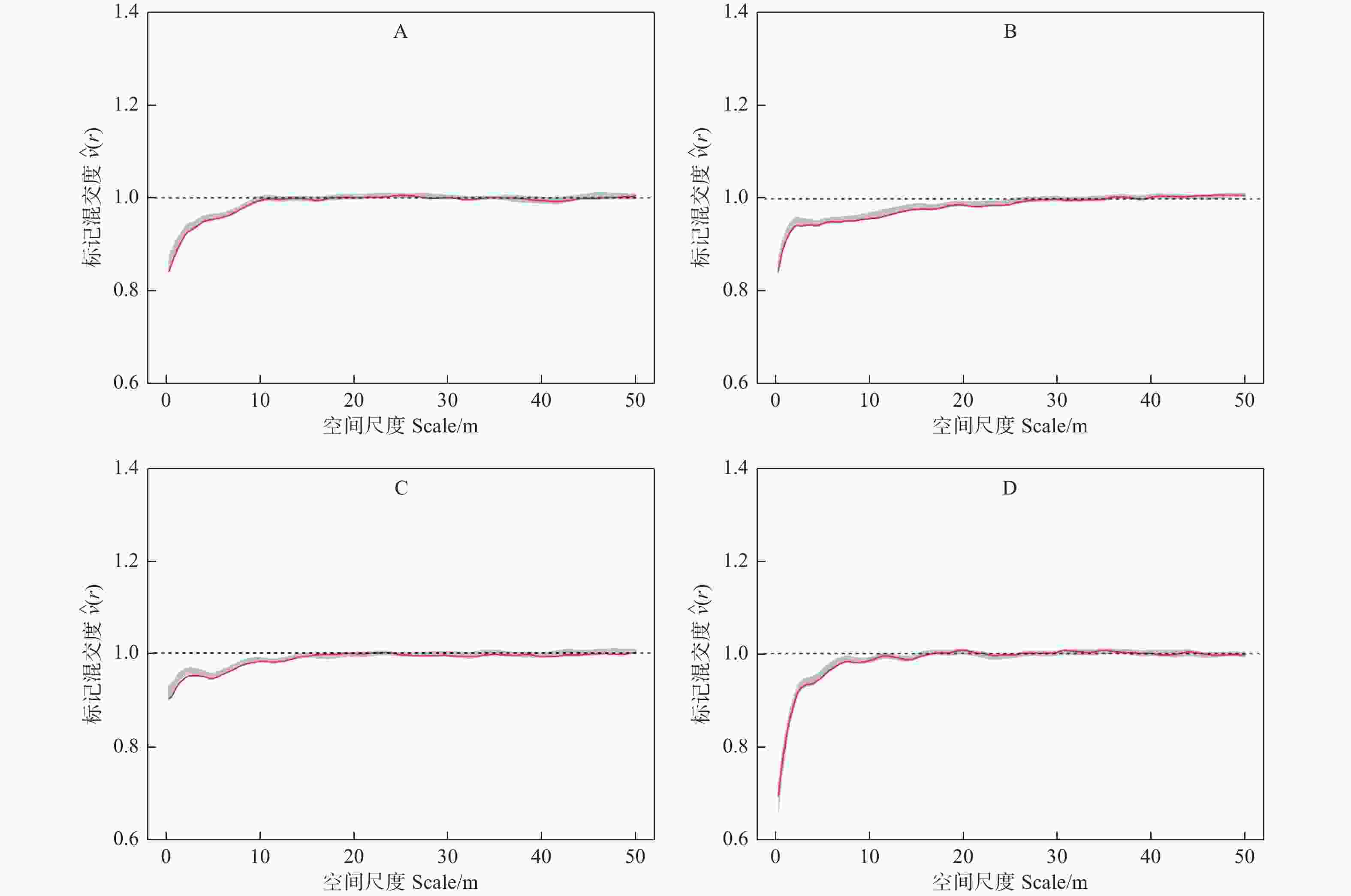
图 3 不同类型标记混交度二阶特征
Figure 3. The second-order characteristics of mark mingling in different types of Korean pine broad-leaved forest
-
本研究分析了不同类型阔叶红松林林木分布格局和标记二阶结构特征,发现不同类型的阔叶红松林的林木分布格局、大小分化标记二阶特征差异明显,特别是水曲柳红松林在小尺度上表现出了明显的小树与大树吸引,小树与小树排斥的特征,明显不同于其他3个类型,这可能与红松阔叶林的发育阶段及干扰程度有关。在4种阔叶红松林中,水曲柳红松林中的红松比例最高,达到了2成,根据李景文的研究,红松阔叶林中阔叶树的伴生作用主要发生在红松发育的前期和中期,在这一范围内,红松的株数极少;随着红松的发育,阔叶树逐步退出群落或者是长寿命的阔叶树与红松之间经过竞争,逐渐达到一种稳定的状态,从而在小尺度上形成大树与小树聚集分布的特征[29]。阔叶红松林的标记混交度特征表明不同类型的阔叶红松林树种分布整体上呈现随机分布,但在小尺度上存在同种聚集的现象,其范围和变化趋势存在明显差异,这进一步说明了不同类型的阔叶红松林处于不同的发育阶段,相同树种聚集程度较高的林分还处于发育的早期阶段,更新主要发生在母树周围;而聚集程度较低的林分是演替的结果,相同树种已经发生自疏现象,其他树种的种子由不同媒介传播,并在一定的范围内更新。根据分析结果可以推测,水曲柳红松林可能处于红松发育的中期或者在历史上受到的干扰程度较小,而其它3种类型的阔叶红松林处于发育的早期或者在历史上受到的干扰程度较大,林木间的自疏作用尚未完成。此外,种内和种间关系、环境的异质性,如水分、土壤、温度、小地形等外部因素也可能是造成林木大小或树种分布呈现不同分布格局的原因,还需要进一步对不同类型阔叶红松林标记二阶特征的形成进行深入探讨和研究。
阔叶红松林是我国东北林区的特有森林类型,在温带针阔混交林类型中占重要地位[30-32]。现有红松阔叶林大多为遭受不同程度的人为干扰后恢复形成的次生林,如何加快红松阔叶林恢复是经营中面临的一个主要问题。邓守彦等认为红松阔叶林在干扰过后,完全可以通过70年的天然恢复接近原始林群落水平,然而,天然林自然恢复是一个漫长的过程,如果辅以合理的人工措施,必然会加速红松阔叶林的恢复[33]。本研究采用的标记二阶特征函数可以对林分不同尺度上的树种和林木大小的分化特征进行细化,其结果对红松阔叶林加速恢复有指导作用,即对于同种聚集程度较高且相同大小林木聚集的林分,可以选择红松优良个体作为培育对象,通过调整其周围较其大的伴生阔叶树种,创造林窗,为红松生长提供充足的营养空间;而对于相同树种聚集且不同大小林木聚集的林分,则主要是调整同种间的资源竞争,伐除相同伴生树种的小树,促进林下红松的更新。当然,在对处于不同恢复阶段的红松阔叶林经营时,还要考虑林分整体的稳定性,需要针对具体林分进行全面的分析。
-
不同类型阔叶红松林的林木分布格局和林木大小分化特征差异明显,树种分布整体上呈现随机分布,但在小尺度上存同种聚集的现象,其范围和变化趋势存在明显差异。不同测试函数标记二阶特征联合分析进一步细化了林木大小分化特征,能够表达处于不同发育阶段阔叶红松林的结构特征,对阔叶红松林加速恢复经营具有一定的指导意义。
吉林蛟河不同类型阔叶红松林标记二阶特征
Mark Second-order Characteristics of Broadleaved Korean Pine Forest
-
摘要:
目的 分析阔叶红松林林分结构的标记二阶特征,探讨不同标记二阶特征函数提供的结构信息和结构形成的生态过程,为阔叶红松林保护、恢复和结构优化调整提供理论依据。 方法 以吉林蛟河4种不同类型阔叶红松林为研究对象,运用单变量双相关函数、标记双相关函数、标记变异函数、标记大小分化度和标记混交度等二阶特征函数,分析树种和林木大小分化空间特征。 结果 不同类型阔叶红松林林木分布格局差异明显,核桃楸、沙松红松林(样地A)、水曲柳红松林(样地C)和核桃楸、色木槭红松林(样地D)在一定的尺度上呈现显著聚集分布的趋势,而核桃楸、水曲柳红松林(样地B)中的林木为随机分布格局;样地A中在距离为 $ r $ =0~50 m的范围内林木标记胸径趋向于小于平均胸径且相似大小林木聚集,其中,在r = 0~8 m和r = 13~33 m的尺度上林木胸径显著小于平均胸径,其他几类阔叶红松林仅在r小于8 m尺度内小于样地平均胸径,其它尺度上林木的胸径大小随机分布;样地B和样地C不同胸径大小的林木呈现空间上不相关的趋势,而样地D在r = 0~9 m的尺度上呈现不同胸径大小的林木聚集分布;4类阔叶红松林不同大小林木的分布并非是完全随机分布的格局,样地A在r = 0~21 m和r = 25~33 m尺度上相似大小的林木聚集在一起,样地B 和样地D分别在r = 4~6 m和r = 0~12 m的尺度上表现出相似大小林木显著聚集的特征,而样地C在r = 0~5 m的尺度上不同大小的林木聚集分布;4类阔叶红松林内树种整体属于完全随机分布,但在一定的尺度上存在同种聚集的现象,样地A、样地B、样地C和样地D相同树种聚集的尺度范围分别为r = 0~10 m,r = 0~25 m,r = 0~12 m和r = 0~8 m。结论 不同类型阔叶红松林标记二阶特征存在明显的差异,与阔叶红松林处于不同的发育阶段及干扰程度有关。标记二阶特征进一步细化了不同尺度上的树种和林木大小的分化特征。 Abstract:Objective To analyze the second-order characteristics of broadleaved Korean pine (Pinus koraiensis) forest in order to provide references for their protection, restoration and structural optimization. Method Taking four types of broadleaved Korean pine forests in Jiaohe of Jilin Province as examples, the single variable double correlation function and second-order characteristic functions of mark double correlation function, mark variation function, mark differentiation, mark mingling were used to analyze the tree species and size differentiation characteristics. Result The distribution patterns of these broadleaved Korean pine forests were significantly different. The distribution patterns of Juglans mandshurica-Abies holophylla-Pinus koraiensis forest (plot A), Fraxinus koraiensis-Pinus koraiensis forest (plot C) and Juglans mandshurica-Acer koraiensis-Pinus koraiensis forest (plot D) showed a significant cluster distribution on a certain scale, while those of Juglans mandshurica- Fraxinus koraiensis-Pinus koraiensis forest (plot B) followed the random distribution. Within the range of r, the DBH of tree mark tended to be smaller than the average DBH and the spatial autocorrelation was positive, especially in the scale of r = 0~8 m and r = 13~33 m. The mark DBH of plot B and plot D showed significant aggregation characteristics of similar size trees on the scale of r = 4~6 m and r = 0~12 m, respectively, while the plot C showed different sizes trees aggregation distribution on the scale of r = 0~5 m. The tree species distribution of the four types of broadleaved Korean pine forests belonged to completely random distribution, but there was the phenomenon of the same species aggregation on a certain scale. The scale ranges of the same species aggregation of plot A, plot B, plot C and plot D were r = 0~10 m, r = 0~25 m, r = 0~12 m and r = 0~8 m respectively. Conclusion The mark second-order characteristics of different types of broadleaved Korean pine forests showed significant difference, which is related to different development stages and degree of broadleaved Korean pine forest. The mark second-order characteristics further refine the differentiation characteristics of tree species and tree size on different scales, which has certain significance for broadleaved Korean pine forest management. -
图 2 不同类型阔叶红松林胸径标记二阶特征
Figure 2. Second-order characteristics of DBH markers in different types of broad-leaved Korean pine forests
图 3 不同类型标记混交度二阶特征
Figure 3. The second-order characteristics of mark mingling in different types of Korean pine broad-leaved forest
表 1 4块样地林分基本特征
Table 1. The basic characteristics of fourdifferent samples
样地
Plot坡度
Slope/(°)海拔
Altitude/m郁闭度
Canopy closure密度
Density/
(trees·hm−2)平均树高
Mean height/m平均胸径
Mean DBH/cm断面积
Basal area/
(m2·hm−2)树种数量
Number of spcices树种组成
Tree compositionsA 9 620 0.90 797 13.7 22.5 31.671 19 3核桃楸2沙松1色木槭1红松4其它 B 8 600 0.85 936 13.8 19.8 28.740 19 3核桃楸3水曲柳1红松3其它 C 9 600 0.9 816 13.6 21.5 29.564 22 3水曲柳2红松1核桃楸4其它 D 9 620 0.85 748 13.1 21.8 27.952 21 2核桃楸1色木槭1榆树1沙松5其它  下载: 导出CSV
-
[1] 惠刚盈, K. v. Gadow, 胡艳波, 等. 林木分布格局类型的角尺度均值分析方法[J]. 生态学报, 2004, 24(6):135-139. [2] Latham P A, Zuuring H R, Coble D W. A method for quantifying vertical forest structure[J]. Forest Ecology & Management, 1998, 104(1-3): 157-170. [3] Wang H X, Zhang G Q, Hui G Y, et al. The influence of sampling unit size and spatial arrangement patterns on neighborhood-based spatial structure analyses of forest stands[J]. Forest Systems, 2016, 25(1): e056. [4] Franklin J F, Spies T A, Pelt V R, et al. Disturbances and structural development of natural forest ecosystems with silvicultural implications, using Douglas-fir forests as an example[J]. Forest Ecology and Management, 2002, 155(3): 399-423. [5] Oliver C D, Larson B C. Forest Stand Dynamics[M]. Wiley and Sons, Inc, New York, 1996, 520 pp. [6] Lei X D, Wang W F, Peng C H. Relationships between stand growth and structural diversity in spruce-dominated forests in New Brunswick, Canada[J]. Canadian Journal of Forest Research, 2009, 39(10): 1835-1847. doi: 10.1139/X09-089 [7] Valbuena R, Packalén P, Martı S, et al. Diversity and equitability ordering profiles applied to study forest structure[J]. Forest Ecology and Management, 2012, 276: 185-195. doi: 10.1016/j.foreco.2012.03.036 [8] Kuuluvainen T, Penttinen A, Leinonen K. et al. Statistical opportunities for comparing stand structural heterogeneity in managed and primeval forests: An example from boreal spruce forests in Southern Finland[J]. Silva Fennica, 1996, 30: 315-328. [9] Spies T A. Forest structure: a key to the ecosystem[J]. Northwest Ence, 1998, 72: 34-39. [10] Ripley B D. Modelling spatial pattern[J]. Journal of the Royal Statistical Society. Series B, 1977, 39: 172-212. [11] Besag J E. Contribution to the discussion on Dr. Ripley′s paper[J]. Journal of the Royal Statistical Society. Series B, 1977, 39: 193-195. [12] Diggle P. Statistical Analysis of Spatial Point Patterns[M]. Academic Press, London, 1983, 148pp. [13] Penttinen A, Stoyan D, Henttonen H. Marked point process in forest statistics[J]. Forest Science, 1992, 38(4): 806-824. [14] Condit R, Ashton P S, Baker P, et al. Spatial patterns in the distribution of tropical tree species[J]. Science (New York, N. Y.), 2000, 288(5470): 1414-1418. doi: 10.1126/science.288.5470.1414 [15] Stoyan D. On correlations of marked point processes[J]. Mathematische Nachrichten, 2010, 116(1): 197-207. [16] Stoyan D, Penttinen A. Recent applications of point process methods in forestry statistics[J]. Statistical Science, 2000, 15(1): 61-78. doi: 10.1214/ss/1009212674 [17] Illian J. Statistical analysis and modelling of spatial point patterns[J]. Technometrics, 2008, 47(4): 516-517. [18] Thorsten W, Kirk A M. Handbook of Spatial Point-pattern Analysis in Ecology[M]. Chemical Rubber Company Press, 2013, 538 pp. [19] 陈科屹, 张会儒, 雷相东. 天然次生林蒙古栎种群空间格局[J]. 生态学报, 2018, 38(10):3462-3470. [20] 郝珉辉, 张忠辉, 赵珊珊, 等. 吉林蛟河针阔混交林树木生长的空间关联格局[J]. 生态学报, 2017, 37(6):1922-1930. [21] Pommerening A, Gonalves A C, Rodríguez-Soalleiro. Species mingling and diameter differentiation as second-order characteristics[J]. Allgemne Forst und Jagdztung, 2011, 182(7): 115-129. [22] Diggle P J. Statistical Analysis of Spatial Point Patterns[M]. Second ed. Arnold, London, 2003, 159pp. [23] Hui G Y, Pommerening A. Analysing tree species and size diversity patterns in multi-species uneven-aged forests of Northern China[J]. Forest Ecology and Management, 2014, 316: 125-138. doi: 10.1016/j.foreco.2013.07.029 [24] Hongxiang W, Pan W, Qianxue W, et al. Prevalence of inter-tree competition and its role in shaping the community structure of a natural Mongolian Scots pine (Pinus sylvestris var. mongolica)forest[J]. Forests, 2017, 8(3): 84. doi: 10.3390/f8030084 [25] Hongxiang W, Hui P, Gangying H Y, et al. Large trees are surrounded by more heterospecific neighboring trees in Korean pine broad-leaved natural forests[J]. Scientific Reports, 2018, 8(1): 9149. doi: 10.1038/s41598-018-27140-7 [26] Gadow K V. Zur Bestandesbeschreibung in der Forsteinrichtung [J]. Forst u. Holz, 1993, 48, 602–606. [27] Grabarnik P, Myllym Ki M, Stoyan D. Correct testing of mark independence for marked point patterns[J]. Ecological Modelling, 2011, 222(23-24): 3888-3894. doi: 10.1016/j.ecolmodel.2011.10.005 [28] Pommerening A, Stoyan, D. Reconstructing spatial tree point patterns from nearest neighbour summary statistics measured in small subwindows[J]. Canadian Journal of Forest Research, 2008, 38(5): 1110-1122. doi: 10.1139/X07-222 [29] 李景文. 红松混交林生态与经营[M]. 哈尔滨: 东北林业大学出版社, 1997. [30] 张玉双, 段文标, 杜 珊, 等. 阔叶红松林主要种群及林隙形成木的空间格局分析[J]. 林业科学研究, 2016,29(3):395-401. doi: 10.3969/j.issn.1001-1498.2016.03.013 [31] 赵中华, 惠刚盈, 胡艳波, 等. 2种类型阔叶红松林优势种群空间分布格局及其关联性[J]. 林业科学研究, 2011, 24(5):554-562. [32] 张春雨, 赵秀海, 郑景明. 长白山阔叶红松林林隙与林下土壤性质对比研究[J]. 林业科学研究, 2006, 19(3):347-352. doi: 10.3321/j.issn:1001-1498.2006.03.016 [33] 邓守彦, 刘万德, 郭忠玲, 等. 不同恢复时期红松阔叶林群落结构与多样性特征[J]. 林业科学研究, 2009, 22(4):493-499. doi: 10.3321/j.issn:1001-1498.2009.04.006 -

 点击查看大图
图(3) / 表(1)
计量
- 文章访问数: 4959
- HTML全文浏览量: 3020
- PDF下载量: 52
- 被引次数: 0


